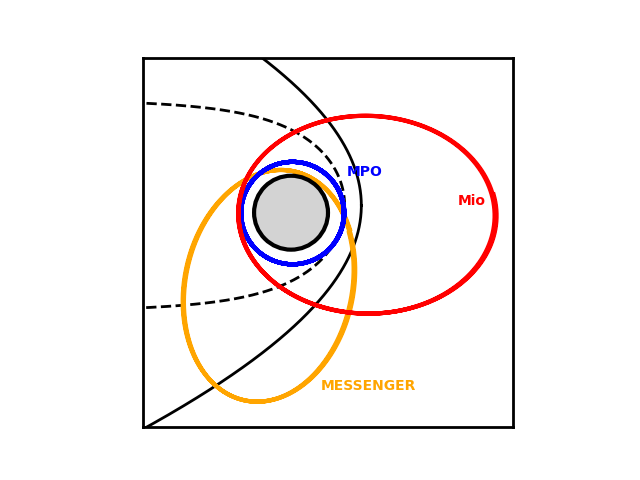
Creating a schematic of spacecraft orbits in Mercury’s magnetosphere

In this example, we talk through how create a to-scale schematic of Mercury’s magnetosphere, inlcuding average boundary locations, and sample orbits from both MESSENGER and predictions from BepiColombo’s MPO and Mio.

import matplotlib as mpl
import matplotlib.pyplot as plt
import spiceypy as spice
from matplotlib.patches import Circle
from sunpy.time import TimeRange

from hermpy.net import ClientSPICE
from hermpy.plotting import plot_magnetospheric_boundaries
from hermpy.utils import Constants as c

# Controls the plot border width
mpl.rcParams["axes.linewidth"] = 2

We start by outlining some times from which to fetch orbits. Here we use TimeRange from sunpy.

bepi_time_range = TimeRange("2026-08-15", "2026-08-16")
messenger_time_range = TimeRange("2012-08-05", "2012-08-06")

We use hermpy.net.ClientSPICE to aid in the downloading a querying of SPICE kernels. We designate specific SPICE kernels to download which we require to get positions for BepiColombo’s MPO and Mio, along with MESSENGER. See here for more details.

spice_client = ClientSPICE()
spice_client.KERNEL_LOCATIONS.update(
    {
        "MESSENGER": {
            "BASE": "https://naif.jpl.nasa.gov/pub/naif/",
            "DIRECTORY": "pds/data/mess-e_v_h-spice-6-v1.0/messsp_1000/data/spk/",
            "PATTERNS": ["msgr_??????_??????_??????_od431sc_2.bsp"],
        },
        "BepiColombo": {
            "BASE": "http://spiftp.esac.esa.int/data/SPICE/BEPICOLOMBO/",
            "DIRECTORY": "kernels/spk/",
            "PATTERNS": [
                "de432s.bsp",
                "bc_sci_v02.bsp",
                "bc_mpo_mlt_50037_20260314_20280529_v05.bsp",
                "bc_mmo_mlt_50038_20251220_20280305_v05.bsp",
            ],
        },
        "BepiColombo Frames": {
            "BASE": "http://spiftp.esac.esa.int/data/SPICE/BEPICOLOMBO/",
            "DIRECTORY": "kernels/fk/",
            "PATTERNS": [
                "bc_sci_v12.tf",
            ],
        },
    }
)

The time ranges defined earlier are used to query the positions for those times in the Mercury-Solar-Magnetospheric (MSM) frame. Those postions are divided by Mercury’s radius (hermpy.utils.Constants) so our plot will be in units of Mercury radii.

with spice_client.KernelPool():
    bepi_times = [t.center.to_datetime() for t in bepi_time_range.split(1000)]
    bepi_ets = spice.datetime2et(bepi_times)

    mpo_positions, _ = spice.spkpos("MPO", bepi_ets, "BC_MSO", "NONE", "MERCURY")
    mpo_positions /= c.MERCURY_RADIUS.to("km").value
    mpo_positions -= c.DIPOLE_OFFSET_RADII.value

    mmo_positions, _ = spice.spkpos("MMO", bepi_ets, "BC_MSO", "NONE", "MERCURY")
    mmo_positions /= c.MERCURY_RADIUS.to("km").value
    mmo_positions -= c.DIPOLE_OFFSET_RADII.value

    messenger_times = [t.center.to_datetime() for t in messenger_time_range.split(1000)]
    messenger_ets = spice.datetime2et(messenger_times)

    messenger_positions, _ = spice.spkpos(
        "MESSENGER", messenger_ets, "BC_MSO", "NONE", "MERCURY"
    )
    messenger_positions /= c.MERCURY_RADIUS.to("km").value
    messenger_positions -= c.DIPOLE_OFFSET_RADII.value

We create our plot, and begin by plotting the above positions. The are in the form of a 2D array, with each column corresopnding to x, y, and z respectively. We define some settings for the axis here as well, to centre the orbits in the panel.

We add labels using matplotlib’s builtin ax.text, and position them manually.

hermpy.plotting.plot_magnetospheric_boundaries can be used to add average bow shock and magnetopause boundary locations to the axis, as determined by Winslow et al. (2013) [link].

Finally, we use matplotlib’s Circle patch to draw Mercury. In the MSM coordinate system, Mercury’s geographical centre is offset from the centre of the coordinate system: the dipole.

fig, ax = plt.subplots()

ax.set(
    xlim=(-4, 6),
    ylim=(-6, 4),
    xticks=[],
    yticks=[],
    aspect="equal",
)

spacecraft_params = {
    "lw": 3,
}
ax.plot(
    mpo_positions[:, 0],  # X
    mpo_positions[:, 2],  # Z
    color="blue",
    **spacecraft_params,
)
ax.plot(
    mmo_positions[:, 0],
    mmo_positions[:, 2],
    color="red",
    **spacecraft_params,
)
ax.plot(
    messenger_positions[:, 0],
    messenger_positions[:, 2],
    color="orange",
    zorder=0,
    **spacecraft_params,
)

ax.text(1.5, 0.8, "MPO", color="blue", weight="bold")
ax.text(4.5, 0, "Mio", color="red", weight="bold")
ax.text(0.8, -5, "MESSENGER", color="orange", weight="bold")

# WARNING: This function will likely change in future versions
plot_magnetospheric_boundaries(ax, "xz", lw=2, zorder=-1)

mercury_circle = Circle(
    (0, -c.DIPOLE_OFFSET_RADII.value),
    radius=1,
    linewidth=3,
    facecolor="lightgrey",
    edgecolor="black",
)

ax.add_artist(mercury_circle)

plt.show()