Creating Multi-panel plots with hermpy

This example demonstrates how to construct multi-panel time series plots using hermpy.plotting.MultiPanel. We fetch one hour of MESSENGER MAG and FIPS data, parse them into their respective data structures, and progressively build up a combined plot.

import xarray as xr
from astropy.table import QTable
from sunpy.time import TimeRange

from hermpy.data import parse_messenger_fips, parse_messenger_mag
from hermpy.net import ClientMESSENGER
from hermpy.plotting import MultiPanel, SpectrogramPanel, TimeseriesPanel

First we must get some data. Here we fetch MESSENGER MAG and FIPS data for a particular time range.

We use hermpy.net.ClientMESSENGER to download MAG and FIPS data for a one-hour window. See here for more details.

c = ClientMESSENGER()
time_range = TimeRange("2011-06-01T00:00", "2011-06-01T01:00")

c.query(time_range, "MAG")
mag_file_paths = c.fetch()

c.query(time_range, "FIPS")
fips_file_paths = c.fetch()

We use Astropy’s Quantity Table (QTable) for time series data, and Xarray’s Dataset for 2D data. These custom parsers are included in hermpy.data, but may be replaced in later versions.

mag_data: QTable = parse_messenger_mag(mag_file_paths, time_range)
fips_data: xr.Dataset = parse_messenger_fips(fips_file_paths, time_range)

print(mag_data)

         UTC           X MSO    Y MSO     Z MSO     Bx     By     Bz
                         km       km        km      nT     nT     nT
--------------------- -------- -------- --------- ------ ------ ------
2011:152:00:00:27.153 4154.624 -736.386 -1295.122  0.184  27.34 64.725
2011:152:00:00:27.653 4155.009  -736.31 -1296.464  0.876 24.996 57.539
2011:152:00:00:28.153 4155.393 -736.234 -1297.805  9.611 28.089 55.024
2011:152:00:00:28.653 4155.778 -736.157 -1299.147  5.836 29.004 55.204
2011:152:00:00:29.153 4156.162 -736.081 -1300.488  7.116 31.518 50.639
2011:152:00:00:29.653 4156.546 -736.004 -1301.829 12.861 25.287 68.678
2011:152:00:00:30.153 4156.929 -735.928 -1303.171 10.287   23.3 61.738
2011:152:00:00:30.653 4157.312 -735.851 -1304.512 16.729 22.473 60.572
2011:152:00:00:31.153 4157.695 -735.774 -1305.853  9.353 22.904  55.89
                  ...      ...      ...       ...    ...    ...    ...
2011:152:00:59:55.203 3658.837   224.82 -8520.415 11.093 13.405 16.675
2011:152:00:59:55.703  3658.56  224.968 -8521.155 11.184 13.404 16.696
2011:152:00:59:56.203 3658.282  225.116 -8521.894 11.185 13.404 16.696
2011:152:00:59:56.703 3658.005  225.263 -8522.634 11.074 13.363 16.772
2011:152:00:59:57.203 3657.727  225.411 -8523.373  11.14 13.356 16.689
2011:152:00:59:57.703  3657.45  225.559 -8524.112  11.22 13.265 16.761
2011:152:00:59:58.203 3657.172  225.706 -8524.852 11.106  13.13 16.843
2011:152:00:59:58.703 3656.895  225.854 -8525.591 11.097 13.133  16.89
2011:152:00:59:59.203 3656.617  226.002  -8526.33 11.222 13.263 16.761
2011:152:00:59:59.703 3656.339  226.149 -8527.069 11.179 13.356 16.746
Length = 7146 rows

print(fips_data)

<xarray.Dataset> Size: 245kB
Dimensions:          (UTC: 199, Energy Channel: 63, Mode: 5317)
Coordinates:
  * UTC              (UTC) datetime64[us] 2kB 2011-06-01T00:23:49.739000 ... ...
  * Energy Channel   (Energy Channel) int64 504B 0 1 2 3 4 5 ... 58 59 60 61 62
  * Mode             (Mode) int64 43kB 0 0 0 0 0 0 0 0 0 0 ... 2 2 2 2 2 2 2 2 2
Data variables:
    Proton Flux      (UTC, Energy Channel) float64 100kB 0.0 0.0 0.0 ... 0.0 0.0
    Non-Proton Flux  (UTC, Energy Channel) float64 100kB 0.0 0.0 ... 0.0 0.0

As MESSENGER MAG data contains both ephemeris and magnetic field data, adding this data as it is to a Panel object will result in an error, as the columns (excluding the time column) have multiple units, and hence can’t be represented on the same axis.

We therefore need to shorten this table to just the columns we want in this Panel object.

mag_data.keep_columns(["UTC", "Bx", "By", "Bz"])

hermpy provides the Panel abstract base class, which is expanded upon in TimeseriesPanel and SpectrogramPanel.

We use a TimeseriesPanel as this matches the data type.

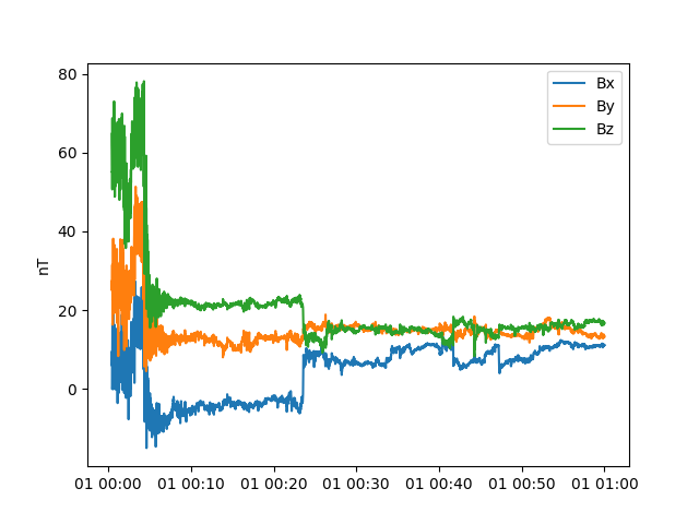
Each panel has a built-in plot function which returns a Figure and Axes for that panel in isolation. plt.show() is called within this function however uou can defer rendering until later by setting .plot(show=False), and then using plt.show() at a later point.

mag_panel = TimeseriesPanel(mag_data)
fig, ax = mag_panel.plot()

Plotting with more than one panel

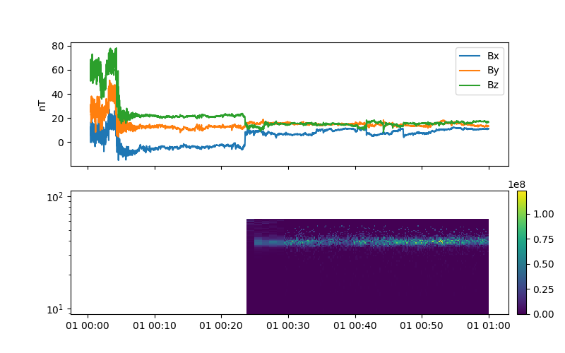
However, the power in Panel objects comes when we go to construct multipanel plots. We can combine Panel objects to construct a multi-panel plot by simply adding them.

Lets make a second panel where we plot the FIPS data. We can combine the two using the addition operator.

proton_flux = fips_data["Proton Flux"]
fips_panel = SpectrogramPanel(proton_flux)

multipanel: MultiPanel = mag_panel + fips_panel
fig, axes = multipanel.plot()

You can also add multipanels to the same effect, and panels can also be added to multipanel objects.

multipanel += multipanel
multipanel.plot()

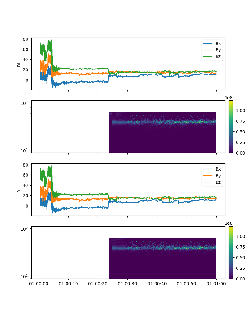
(<Figure size 800x1000 with 4 Axes>, array([<Axes: ylabel='nT'>, <Axes: >, <Axes: ylabel='nT'>, <Axes: >],
      dtype=object))

multipanel += mag_panel
multipanel.plot()

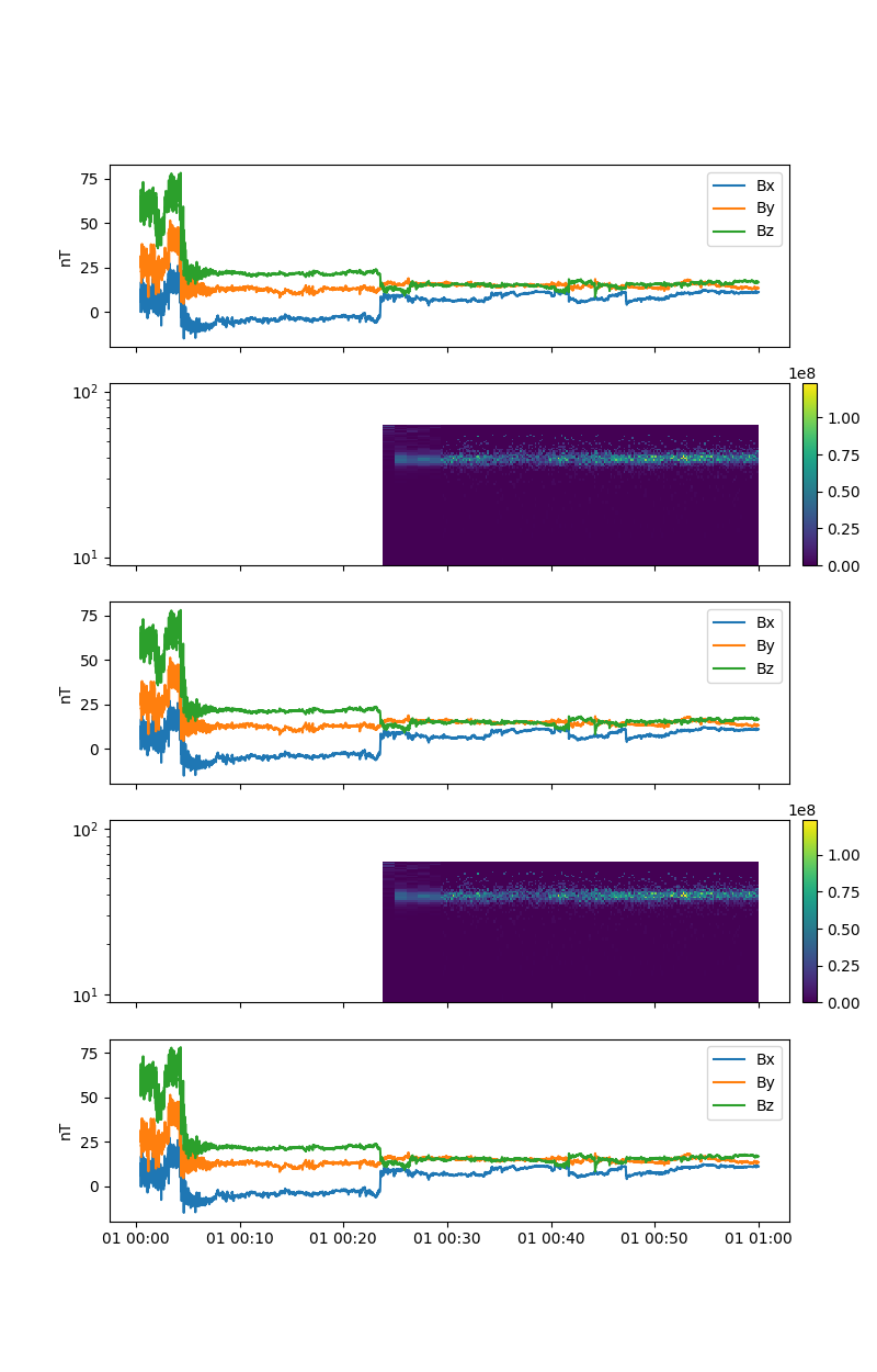
(<Figure size 800x1250 with 5 Axes>, array([<Axes: ylabel='nT'>, <Axes: >, <Axes: ylabel='nT'>, <Axes: >,
       <Axes: ylabel='nT'>], dtype=object))