
Note
Go to the end to download the full example code.
Plotting an orbit of MESSENGER MAG#
In this example, we showcase the downloading, and minimal analysis required to plot a single orbit of MESSENGER MAG data.
import datetime as dt

import matplotlib.pyplot as plt
from matplotlib.dates import DateFormatter
from sunpy.time import TimeRange

from hermpy.data import (
    add_field_magnitude,
    parse_messenger_mag,
    rotate_to_aberrated_coordinates,
)
from hermpy.net import ClientMESSENGER, ClientSPICE
from hermpy.utils import Constants as c
Downloading data#
We use hermpy.net.ClientMESSENGER to access MESSENGER data. See here
for more details.
start_time = "2012-04-01 05:00"
time_range = TimeRange(start_time, dt.timedelta(hours=8))

downloader = ClientMESSENGER()
downloader.query(time_range, "MAG 60s")
files = downloader.fetch()
Files Downloaded:   0%|          | 0/1 [00:00<?, ?file/s]

MAGMSOSCIAVG12092_60_V08.TAB:   0%|          | 0.00/223k [00:00<?, ?B/s]

MAGMSOSCIAVG12092_60_V08.TAB:   0%|          | 1.02k/223k [00:00<00:31, 7.07kB/s]

MAGMSOSCIAVG12092_60_V08.TAB:  20%|██        | 45.7k/223k [00:00<00:01, 153kB/s]


Files Downloaded: 100%|██████████| 1/1 [00:00<00:00,  1.41file/s]
Files Downloaded: 100%|██████████| 1/1 [00:00<00:00,  1.41file/s]
Parsing the data#
The above code-block downloads MESSENGER MAG data in their raw .TAB
format. hermpy.data implements useful routines to parse these data into
an Astropy QTable.
data = parse_messenger_mag(files, time_range)
data = add_field_magnitude(data)

print(data)
         UTC          N Observations  X MSO   ... SD(Bz)        |B|
                                        km    ...   nT           nT
--------------------- -------------- -------- ... ------ ------------------
2012:092:05:01:00.000           1200 5711.456 ...  3.405 19.237045563183553
2012:092:05:02:00.000           1200 5723.014 ...  3.136 19.052457085635965
2012:092:05:03:00.000           1200 5734.404 ...  3.151    19.122289245799
2012:092:05:04:00.000           1200 5745.625 ...  3.686 18.583599758927225
2012:092:05:05:00.000           1200 5756.673 ...   3.95  18.75248932808655
2012:092:05:06:00.000           1200 5767.549 ...  3.199 19.280475227545615
2012:092:05:07:00.000           1200  5778.25 ...  3.918  19.08125158368811
2012:092:05:08:00.000           1200 5788.774 ...  3.106 19.000645962703476
2012:092:05:09:00.000           1199 5799.119 ...   3.11 19.178216131851265
                  ...            ...      ... ...    ...                ...
2012:092:12:50:00.000           1200  570.035 ...  0.691 14.164434616319847
2012:092:12:51:00.000           1200  597.002 ...  1.758 14.104693332362814
2012:092:12:52:00.000           1200  623.956 ...  0.924 14.402472461351904
2012:092:12:53:00.000           1200  650.899 ...  1.845 14.293685528931997
2012:092:12:54:00.000           1200  677.828 ...  1.069 14.332983325183909
2012:092:12:55:00.000           1200  704.745 ...  1.231  14.09889814843699
2012:092:12:56:00.000           1200  731.648 ...  0.757   14.0850225061943
2012:092:12:57:00.000           1200  758.537 ...  0.844 13.985270859014495
2012:092:12:58:00.000           1200  785.412 ...  1.334 14.032536335246027
2012:092:12:59:00.000           1199  812.271 ...  0.846 14.132853427386841
Length = 479 rows
Converting to MSM Coordinates#
Note that these data contain the position and magnetic field values in Mercury-Solar-Orbital (MSO) coordinates. We should convert to Mercury-Solar-Magnetospheric (MSM), where the origin is co-situated with Mercury’s dipole. We can do this by adjusting the z-axis by the dipole offset: 479 km (~0.2 R) [1].
Note
Note that while we will not plot any position data in this example, we felt it fit to include these instructions here.
data["X MSM"] = data["X MSO"]
data["Y MSM"] = data["Y MSO"]
data["Z MSM"] = data["Z MSO"] - c.DIPOLE_OFFSET.to(c.MERCURY_RADIUS)
Aberrating the reference frame#
Additionally, these coordinate systems point the x-axis
towards the Sun. Often it is also useful to rotate (or ‘aberrate’) the
reference frame such that the x-axis points into the solar wind flow.
The convention to denote aberrated frames is by using
primed-notation: '.
Aberration is a calculation based on the velocity of Mercury, and an assumed
solar wind velocity of 400 km/s. To determine these, we must load some spice
kernels. The built-in kernels to hermpy.net.ClientSPICE are sufficient to
compute this. See here for more details.
spice_client = ClientSPICE()

with spice_client.KernelPool():
    data = rotate_to_aberrated_coordinates(data)

print("Columns:")
for column in data.columns:
    print(column)
Files Downloaded:   0%|          | 0/8 [00:00<?, ?file/s]
Files Downloaded:  12%|█▎        | 1/8 [00:00<00:01,  4.00file/s]
Files Downloaded: 100%|██████████| 8/8 [00:00<00:00, 25.41file/s]
Columns:
UTC
N Observations
X MSO
Y MSO
Z MSO
Bx
By
Bz
SD(Bx)
SD(By)
SD(Bz)
|B|
X MSM
Y MSM
Z MSM
X MSO'
Y MSO'
Z MSO'
X MSM'
Y MSM'
Z MSM'
Bx'
By'
Bz'
Aberration Angle
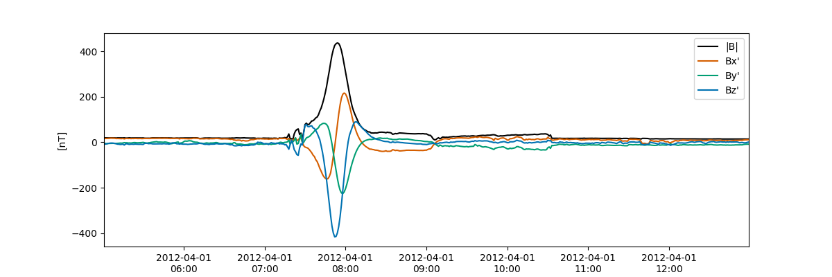
Plotting#
Here we use colours from a 7-colour palette by Wong (2023) [2]
Additionally, it is nice to set a custom DateFormater to be
less ambiguous about the y-ticks.
fig, ax = plt.subplots(figsize=(12, 4))

vars = ["|B|", "Bx'", "By'", "Bz'"]
colours = ["black", "#D55E00", "#009E73", "#0072B2"]

for var, colour in zip(vars, colours):
    ax.plot(data["UTC"].to_datetime(), data[var].value, color=colour, label=var)

ax.legend()
ax.margins(x=0)
ax.set_ylabel("[nT]")
ax.xaxis.set_major_formatter(DateFormatter("%Y-%m-%d\n%H:%M"))

plt.show()
References#
Total running time of the script: (0 minutes 3.662 seconds)